


Written by Bill Comeau
This is a guide to the 2020 SKATR player evaluation tool. It includes instructions on its use and details behind the 24 NHL statistics it displays.

1. Introduction
A skilled player will make hundreds of instant decisions and subtle elite movements in a game. I wish we could capture all of that, but it’s beyond our abilities. Artistry defies numbers and just looking at numbers will never describe the full picture. But what we can do is synthesize all the play-by-play statistics and try and gauge how a skater’s talent impacts the results.
“We feel that we’ve got an abundance of skill and the ability to make plays which ultimately lead to having the puck which ultimately leads to scoring goals at a high rate. That is the object of the game, ultimately.”
– Sheldon Keefe on January 10, 2020.
This statement by Keefe is at the heart of SKATR’s philosophy. The focus is on player skills and results. Whether it’s shooting percentage, the rate of passing to set up shots, getting into more expected goal situations, suppressing chances against, driving play up ice, or drawing penalties — that is the focus.
Below are my two favourite hockey players: Connor McDavid and Auston Matthews. They were the inspiration for SKATR.
STOP WHAT YOU'RE DOING AND WATCH THIS CONNOR McDAVID GOAL! 😳🚨⭐️@EdmontonOilers | #EDMvsTOR pic.twitter.com/0ecTLmQ7kd
— NHL on NBC (@NHLonNBCSports) January 7, 2020
The hands and the celly. A Matthews specialty. #LeafsForever pic.twitter.com/EJwuaUpld0
— Maple Leafs Hotstove (@LeafsNews) December 18, 2019
Here are their SKATR profiles. The beauty lies above in those clips; SKATR simply tries to add a layer of insight.

McDavid and Matthews – Some Quick Takeaways
To help us get started and to provide a brief sample of interpreting SKATR, here are a few takeaways from the above chart. [Percentiles are shown in square brackets.]
- In the context section, we can see that McDavid is at the top in ice time usage [100], like Matthews [98]; TOI vs Elite competition [86] is tougher than Matthews [69] and things are rocking with McDavid on the ice with a very high on-ice shooting percentage [91] vs [79] for Matthews. I suspect that this five-man shooting percentage is greatly influenced by the best player in the world opening up space and finding teammates. However, McDavid plays on a team with weaker play-driving teammates as seen by a [42] CF% vs [93] for Matthews.
- Connor boosts on-ice expected goals for him and his teammates at a high rate [92] but that explosive offense is countered by elite competition that drives plenty of strong expected goal counterattacks against [9]. Auston, in contrast, has very good ‘two-way’ relative to teammate numbers this season, though he doesn’t face elite forwards as often, in part due to Tavares being a second top-line center on the team.
- Offensively, McDavid’s speed threat, play-making, and vision produce a lot more primary assists [94 to 66] and the secondary assists gap is even more pronounced [88 to 30]. But Matthews has a higher shooting % [91 to 80] and shoots much more often [97 to 63]. Although they have a similar rate of expected goal opportunities [92 and 91], Matthews scores more frequently [99 to 87].
- While SKATR focuses on 5-on-5 play, special team percentiles are shown in the lower corner to add context on their overall game. There we can see that McDavid is at the 100th percentile in power play points per 60 while Matthews is at the 89th.
That’s just a sample of what you can draw out of one SKATR chart. You can see the depth of what SKATR can provide. If you need the actual raw statistics, they are found in another part of the tool under the “Stats” tab.
In McDavid and Matthews, you have the fastest — and I believe greatest — all-around offensive hockey player in the world opening up opportunities and generating points at an elite rate, and you have perhaps the greatest pure goal-scorer of this generation.
The two video clips capture part of this story while SKATR tries to add insights drawn from numbers that capture every single five-on-five shift. They are very different players, but both are also very special.
Design and Philosophy
The main goal of SKATR is to describe a player’s results as fairly and consistently as possible. That means:
-
-
-
- restricting focus to the 5v5 hockey game
- adjusting for score and venue effects
- using rates per 60 minutes to adjust for playing time
- only looking at players with 100+ minutes ice time at 5v5
- providing the context surrounding the player’s deployment
- looking beyond highly variable goals and points to more stable underlying results
- selecting a representative cross-section of useful hockey statistics
- avoiding the use of 5-man statistics to describe a single player (eg +/-, CF%, xGF%)
- ranking players at their position (SKATR uses percentiles)
-
-
When you look at any SKATR chart, you are looking at percentile rankings — not the raw statistic. The percentiles are based on 5v5 “per 60” statistics — not raw counts. The labels are percentiles, the colours are based on percentiles, and even the lengths of the bars are based on the percentiles.
It may seem highly redundant, but it’s the percentiles I want to drill home and convey in SKATR in an already-complex chart — not some arcane, forgettable four-decimal-place numbers. Auston Matthews has not scored 99 goals in the above chart, but he is ranked at the 99th percentile among 100+ minute forwards in 5v5 goals per 60 minutes (1.66 goals/hour in this example).
In comparing skaters, always keep in mind that the statistics chosen may overlap (e.g goals and points). Also, keep in mind that they will vary in importance. Goals are more important than shots, for example.
Data Sources and Credits:
None of this work would be possible without the support of these free access data sources. I encourage SKATR users to pay them a visit and support them.
– Natural Stat Trick for individual, on-ice, and bio stats
– MoneyPuck for expected goal and game score stats
– PuckPedia for contract information
– PuckIQ for TOI vs Elite competition
– Corsica for Quality of Teammate and TOI%
– NHL play-by-play data for relative to teammate, xGF%, CF% calculations
– Tableau Public free-use visualization software
2. Using SKATR
You may want to open up SKATR and follow along. It can be found at this Advanced Statistics page.
General tips:
SKATR is generated by Tableau visualization software. There are several important user controls on the lower right:

- The three arrows on the left allow you to undo, redo, or reset your selections.
- The next icon to the right lets you share the link or embed SKATR.
- The second icon from the right let’s you download your displayed SKATR to an image, PDF, or PowerPoint.
- The most important option is on the right – it displays SKATR in full screen. SKATR usually needs to be opened to full screen to avoid a squished display.
Check the note at the bottom to see when it was last updated. This is also where you will find links to this Guide and the Glossary.
Besides the MapleLeafsHotStove.com home website, you can also find SKATR and some of my other viz at my Tableau Public Gallery link: bit.ly/Billius27

2.1 Menus
To select players, use the six drop-down menus located beneath the title. Start from the middle. Select a position first (forward or defenseman), and then you can optionally select their July 1, 2020 contract status (restricted free agent, unrestricted free agent, or signed). This comes in handy as the trade deadline approaches and teams are known to look for rental players. Setting to UFA will give you a dropdown list of pending July 1st UFA’s.
Next select the player and season (2019-20, 2018-19, and 2018-20) you want for both the left and right sides. Note that only relevant players are listed in the player dropdown menu; if you see a blank chart, check your middle-menu choices. Also, note that you can choose the same player for both sides and vary the season. I would recommend using the 2018-20 season choice for players with low minutes. The more minutes you have, the more stable the picture of that skater — although skaters who change teams will often show changes in their performance.
Once your choices are made, the SKATR header strips and bar charts will appear for each player. If you go to the top tabs and click “Solo”, you will see that Solo is a full-page version of the left-hand-side player chart.
2.2 Percentile Bars
There are 24 5v5 statistics in SKATR, divided into four categories: five Box Score, six Underlying, six Relative to Teammates, and seven Context statistics. Each one has a coloured percentile bar with the percentile labeled on the bar. A percentile is simply a way of taking a statistic like 1st Assists/60 and ranking players from top (100) to bottom (0). If there are about 500 forwards, roughly five players will have a 100th percentile ranking and five will have a zero ranking.
You will also see vertical dividers at the 20th, 40th, 60th, 80th, and 100th percentiles. These can be used as a rough visual guide for first, second, third, fourth, and replacement-level line performance for each statistic. The percentile bars are also shaded in 10 colours — one for each 10 percentile range, 5 red and 5 blue.
Mitch Marner is near the top of the league’s forwards when it comes to 5v5 primary assists per hour, so he has a “97” on his long darkest blue “1st Assists” bar. The percentiles are calculated based on the specific position and season you select and SKATR only looks at qualified players — in this case, forwards with 100 or more 5v5 minutes in 2019-20.
If you hover over a bar, a pop-up will provide a description and guide you to the Stats tab if you are interested in the actual statistic.

2.3 Special Team Meters
Special team “meters” are included in the bottom corners of SKATR.
They include vertical percentile bars for the penalty kill and power play.

The penalty kill percentile uses “xGA/60 Rel” from Natural Stat Trick, or in long-form: relative to team expected goals against per 60 minutes on the penalty kill. The more a player reduces the expected goals below his team’s average, the higher his percentile goes. Some caution is needed because a top penalty killing unit will face more set playoff starts and the opponent’s top power play unit.
For the power play, the percentile of points per 60 is used.
In the chart above, Marner and Nylander are at the 97th and 70th percentiles when it comes to power play points per 60. Marner is also at the very low 1st percentile on the penalty kill “xGA60 Rel” metric with a value of +2.49 per 60 relative to his team (found my hovering).
Only players with 50+ minutes of time on the penalty kill or power play are reported, otherwise that special team will remain blank as it is for Nylander above.
The actual special team statistics can be found by hovering over the meters.
2.4 Customizing the Display
There is one trick that comes in handy if you want to display a subset of SKATR’s 24 statistics. All you need to do is click on a label — e.g. “On-Ice Sh%” — wait for a popup window, and then click “Exclude” to exclude it from the chart. You can do this repeatedly to simplify the chart you want to share.
Example: remove On-Ice Sh%
 Now it’s removed.

2.5 Stats Report
The “Stats” tab at the top of SKATR takes you to a report showing the 5v5 per 60 statistics used in calculating the percentiles for the players and seasons selected on the main dashboard.
These are the rate statistics that were used to rank the players and create percentiles.

2.6 Miner
SKATR can compare two players, but sometimes more than two need to be explored and compared. Miner can be found in the top tabs and is basically an extended version of SKATR but with the table rotated, to allow a list of players instead of just one.
The 24 statistics are now listed across the top and instead of percentile bars, each percentile is shown in a single coloured cell. There is one row now for each player. The colours match those used in SKATR — dark blue are the best (highest percentiles) and dark red are the lowest percentiles.You can either review a team by position by using the Team and Position dropdown menus on the upper right, or you can customize your search across all teams.
In the example below I decided to look at 2019-20 results for right-handed defensemen who will be UFA’s on July 1st, 2020. I further narrowed the search by using the sliders to select 30+ year-olds and who have a relative to teammate expected goal share that puts them in the top 50%.
I used the sort menu in the upper left to sort players by 5v5 Skatr Score percentile. The result is a list of RD, we can see that Kevin Shattenkirk and Alex Pietrangelo are at the top of this group.
We can also use the context results to identify defensemen who play up or down in the lineup and face higher or lower competition. For example, we can see that three Kevin Shattenkirk’s context needs to be considered, since he is only at the 36th percentile when it comes to his percentage of ice time versus elite forwards.

Here’s another example, this time using the Team and Position menus. It also shows how the customization explained in section 2.3 can help simplify the table by reducing the number of statistics (columns) . If I wanted to write an article about the second tier of Leafs wingers, this would be helpful.
There is a lot to consider in a table like this but we can see how rookies Ilya Mikheyev and Pierre Engvall have entered the conversation as top 6 winger candidates (Ilya is facing a long injury rehab now) and how suggestions to trade Andreas Johnsson may be premature.

Now let’s go over the meaning of the 24 SKATR statistics.
3. Understanding SKATR’s Statistics
Note: All statistics are 5v5* and are converted to per 60-minute rates. I won’t be repeating that for every definition. * with the exception of the power play and penalty kill meters in the lower corner of SKATR.
Below is a correlation matrix for 2019-20 for forwards showing how pairs of SKATR statistics are correlated with each other. The bottom diagonal uses coloured circles to highlight the correlations (blue are positive, red are negative correlations) and the top diagonal shows the actual correlation values.
A correlation (r) ranges from -1 to +1 and simple shows how strongly one statistic is related to another. An r = 0 means they are totally unrelated, r = -1 means that one trends perfectly down as the other trends perfectly up, r = +1 means they are perfectly related.
The statistics are in the same order as SKATR.
The main point here is to not add up bars and reach some “summary” conclusion, these statistics are mostly inter-related. But you can also look at these correlations to gain a deeper understanding of how to interpret SKATR.
Correlogram

3.1 Box Score Statistics
3.1.1 “Skatr Score” (New)
Why the change?
As of February 2020, Skatr Score has replaced the original 5v5 Game Score.
I decided to take this step because the original game score pulled from the corsica database is a little outdated (it is not the one used by Dom L. at The Athletic anymore) and because I wanted to incorporate additional statistics that SKATR has at the cumulative YTD or season level that individual game box scores do not, such as relative to teammate metrics and estimated shot assists.
I also wanted to let the data decide what should be included. This meant skipping measures that do not impact goals for or against in any significant measurable way, like hits.
Method and Key Variables
The new score is customized for SKATR and is based on separate forward and defense multiple regression models for October 2018 – present. Only those measures that were statistically significant in explaining the variation in on-ice goal differentials were kept in the models. Descriptions of the variables can be found in a later section of the Guide.
Skatr Score is still correlated to the old 5v5 game score though it uses a different scale based on goal differential. The plot shows the new forward Skatr Scores on the vertical axis plotted against Game Score on the horizontal (r=.89).

 On the right are the SKATR statistics that go into each model’s score.
The final predictor variables in the regressions are fairly intuitive, obviously goals and assists directly impact a team’s goal differential at 5-on-5. For that reason, a score like this will be highly correlated with points. However, primary assists did not show up for defensemen whereas their more common contribution as “secondary assisters” did.
Besides these box-score statistics, the score also factors in individualized underlying estimates like shot attempt and shot assist rates as well as relative to teammate metrics. The intention is to better capture two-way and defensive play. Shot attempts (ie shots) did show up for defensemen (which makes sense) while forwards had an extra consideration based on their ability to push expected goals (xGF per 60) relative to teammates (again makes intuitive sense).
You will also see that the “relative to teammates expected goals against per 60” is in both the forward and defense models. This statistic is one of the few measures of player defense and so it’s important when we are trying to account for on-ice goals for and against.
Importance of Variables
Here are the relative importance weights for each variable in the models.


The importance weights are tied to how each predictor variable improves the fit of the multiple regression model (improvement in adjusted R-squared when the variable is the last to enter the model).
The regression process picked the variables and the weights. But there are some things worth noting:
- Relative to teammate expected goals against (rtmxga60) is the most important forward variable, which might not seem intuitive until we remember that the model is predicting on-ice goal differential, not just goals for.
- Estimate shot assists (esa/60) is most important for defensemen – again because we are predicting goal differential and not just defense.
- Goals and assist rates show up in both models as expected. For defensemen, the secondary (A2) assists are in the model but primary assists (A1) are not. This is due to the sporadic nature of primary assists for defenseman versus forwards where it is much more important. (Most defensemen assists are secondary.)
Besides the two regression models, I added a penalty differential to the score by applying power play league average goals for and against per 60.
Top-Ranked 5v5 Players Based on Skatr Score
Below are the YTD 2019-20 top-ranking forwards on Skatr Score, using the Miner report. Artemi Panarin and Brad Marchand lead the rankings and you can see how highly they score on the seven forward model variables (plus penalty +/-). The surprise is Nick Bonino who is having an outstanding season and also has very high percentiles at 5v5, although the context also tells us he plays in a role where he faces less top competition.
There are a couple of things to keep in mind:
-
-
- players with lower minutes (say under 500) can temporarily rank unusually high or low on these rate-based statistics
- context metrics are not factored into the Skatr Score (eg Bonino)
-

3.1.2 Points, Goals and Assists
Points = Goals + 1st Assists + 2nd Assists.
1st assist = the pass leading directly to the goal, also known as the primary assist. It is generally more indicative of forward play-making talent than a second assist.
2nd assist = the secondary assist, often considered less useful in understanding forward talent since it is less reliable in predicting future forward performance and is less directly tied to goals. It is included mostly because it can help describe the offensive side of defensemen who are much less likely to generate primary assists.
You can read more about secondary assists in this Eric Tulsky article.
3.2 Underlying Statistics
These statistics are ones that don’t show up directly on the scoreboard but are important in understanding a player’s individual performance. They can also be more stable indicators than the ups and downs linked to scoring ‘luck’ and can help point to specific talents, such as getting into scoring position, playmaking, and shooting.
3.2.1 Shots aka Shot Attempts
Individual shot attempts (iCF/60). This includes an individual player’s blocked shots, missed shots, shots on goal that were saved, as well as shots that became goals. I generally refer to shot attempts as shots as do many in the analytics community.
Many of the shot-based stats in SKATR have historically been named after Jim Corsi, a coach who was tracking shots for his goalie and somehow got stuck with the label. But the term I prefer for any stat is one that simply says what it is and avoids any needless confusion. It’s also why I won’t call unblocked shots “Fenwick”.
The most important thing to know about shot stats is that because they provide a much larger sample size of events than the much rarer and more random actual goals scored, they are often more predictive of things like future team goal differential.
3.2.2 Estimated Shot Assists
Also referred to as “esa/60” in SKATR. “esa/60” is relatively new and is based on large samples of manually tracked ‘microstat’ passing data. Just like goals have assists, shots have shot assists, too. It’s just that no one ever manually tracked them in a significant way until recently. That work has mostly been done by Corey Sznajder, Ryan Stimson, and others.
The regression formula I am using to calculate estimated shot assists was developed by Alan Wells (@Loserpoints). That regression predicted eSA based on passing data samples and known classic stats, namely assists, individual shots (iCF), and on-ice shots (CF).
eSA/60, though not perfect, expands our knowledge about a player’s general passing skill activity — looking at both individual shots and eSA is analogous to looking at goals and assists only over a wider band of game activity. The combination of shots and eSA/60 is called “Estimated Shot Contributions” and has been shown to be more predictive of future point scoring than a player’s actual points. You’ll find those two percentile bars next to each other in SKATR for that reason.
More on estimated shot assists can be found here: https://hockey-graphs.com/2017/12/12/estimating-shot-assists/.
3.2.3 Expected Goals
This is individual expected goals (ixG), not to be confused with on-ice xG measures later in SKATR. The ixG estimates are based on MoneyPuck’s expected goal model that takes into account the probability of scoring a goal for each unblocked shot. (Blocked shots have no recorded rink location.)
Expected Goals factors in shot location and other elements like the time and angle between shots, and rebounds. There are several ‘xG’ models available, I’m using the MoneyPuck one because I frankly consider it to be the best. To calculate a player’s ixG, their expected goal probability for each unblocked shot is summed to give total expected goals for a player.
Let’s look at a simple example: If I have two shots at 5v5 in a game, one from the blue line with a 2% probability of scoring and one from the inner slot with a 23% chance of scoring, my total xG is .02 + .23 = .25 expected goals for the game. If I played 15 minutes at 5v5, my ixGF per 60 would be (60/15) x .25 or 1.0. Not all shots are created equal and xG stats help to adjust for the danger of shots taken.
But xG does not take into account an individual player’s shooting talent, any pre-shot movement like a cross-slot pass, or who the goalie is. It’s an average expectation given the history of over a million shots and all the known trackable factors surrounding those shots.
More information on the MoneyPuck model can be found here. There you can find a list of the many factors used to predict a shot’s xG. You can also explore a player’s shot locations and expected goal statistics in the GameShots viz, which can also be found in the MLHS Advanced Statistics page where SKATR resides.
3.2.4 Shooting Percentage
Shooting percentage is the percentage of individual shots on goal by a player that result in goals. In fact, it is very highly correlated to goals, with a correlation coefficient of r=.85. It tends to randomly fluctuate up and down during a season for a skater, just like goal scoring streaks and slumps.
Shooting Percentage has several components – it is a function of the expected goal probability for an average player given the shot location and other factors, as well as underlying “shooter talent”, goalie quality, and plain old random luck, even shots off the cross-bar.
Because of this volatility, it is normally unwise to read too much into a player’s shooting percentage over a short timeframe. There are elite shooters such as Auston Matthews, who can consistently achieve a high shooting percentage, but in general, players will bounce around from month to month or season to season and will tend to “regress to the mean” over time. A good example is William Nylander, who was at the 16th percentile last season (5.3%) and is currently at the 83rd percentile this season (14.1%).
You can read more on shooting percentage and regression to the mean here.
3.2.5 IPP
IPP stands for Individual Point Percentage: the percentage of 5v5 goals for that player’s team while that player was on the ice and where that player earned a point.
IPP = (Player Points at 5v5) / (Goals For at 5v5)
On average, a SKATR forward right now has a 2019-20 IPP of around 64.6%. This means he has scored a point on 64.6% of goals scored while they were on the ice at 5v5 (defensemen averaged 32.6%). Forwards who are much more involved in their team’s scoring will score higher on IPP. One example is Leon Draisatl who has been in on 86.8% of his team’s 5v5 goals so far this season.
Sometimes a player will have an abnormally “lucky” year. Players who aren’t normally great point producers but have a high IPP percentile can be investigated at Natural Stat Trick to see if it is out of pattern with their historical levels.
For example, Jake Virtanen has an IPP of 95%, which places him at the 98th percentile among NHL forwards. Harman Dayal of The Athletic looked into Jake Virtanen’s high IPP in a paywall article, and here is what he discovered:
“The ratio at which Virtanen is collecting points on the goals he’s on the ice for is simply unsustainable. He’s fluctuated between a much more realistic 55 and 68 percent IPP in other seasons.”
You can read another article on using IPP here by Travis Yost.
3.2.6 Penalty +/-
Sometimes referred to as “penalty differential”. It’s the difference between 5v5 penalties drawn and 5v5 penalties taken by a player. Analysis has shown that this is a repeatable ‘talent.’ Since power plays are roughly four times as likely to generate a goal, it’s an important player trait. In fact, most WAR models will include this as a separate player component.
Players with a negative statistic (and lower percentile) generate more power plays for the opposing team. Like many results, the context can affect the result. A defenseman playing against top forward lines is more apt to take penalties. (As a rule, defensemen and forwards should never be compared in SKATR anyways, for obvious reasons.)
3.3 Relative to Teammate Statistics
On-ice statistics cover what is happening on the ice at 5v5 for all five players. A shift with five teammates would be the same for each teammate on that shift. That is why it is important to try and separate out the impact each player and teammate has on on-ice statistics such as xGF% and CF%.
If you skip down to section 3.34, “Relative to Teammates CF%”, you will find an example of how the basic calculations are made. The CF% approach is repeated for every relative to teammate statistic in this section.
In SKATR the calculations are a little more involved, I will touch on them here for those interested.
More on the Relative Teammate Methodology in SKATR
I chose to adjust for teammates with less than 100 minutes of ice time away from a player to remove “noise”. Some (small) team effects were also adjusted for. These adjustments were largely based on an article by Evolving Wild.
I also decided to use MoneyPuck expected goal estimates at the unblocked shot level, so in effect every play-by-play shot and every player-shift has been recalculated at the play-by-play level to create the relative to teammate statistics covered in this section.
Most hockey sites like Natural Stat Trick do not report relative to teammate statistics. It’s important to note that relative to team statistics are easier to compute but are less ideal and since SKATR isn’t processing nightly, I have chosen to use the more precise teammate version. Relative to team issues are explained in the above-linked article.
You could also go further down this road and explore Regression/Regularized Adjusted Plus-Minus approaches or the use of regression methods in the isolated heat maps of Micah McCurdy.
3.3.1 Relative to Teammates Expected Goal Share
Relative to teammates xGF% is the change in expected goal share when a player is on the ice at 5v5 compared to the xGF% when his teammates play without him in the same games.
A player who is able to aid his teammates in creating more 5v5 expected goals than opponents will score higher on this statistic. The underlying shot xG estimates are from the MoneyPuck model.
3.3.2 Relative to Teammates Expected Goals For
Relative to teammates “expected goals for” is the change in xGF for a player’s team when a player is on the ice compared to the xGF when his teammates play without him in the same games.
A player who is able to aid his teammates in creating more 5v5 expected goals on offense will score higher on this statistic. The underlying shot xG estimates are from the MoneyPuck model.
3.3.3 Relative to Teammates Expected Goals Against*
Relative to teammates expected goals against is the change in xGA for a player’s team when a player is on the ice compared to the xGA when his teammates play without him in the same games.
A player able to prevent fewer 5v5 expected goals against on defense will score lower on this statistic. This is sometimes referred to expected goal suppression and is the most important defensive statistic in SKATR. The underlying shot xG estimates are from the MoneyPuck model.
*Note that the percentile shown in SKATR is set up so that it gets closer to 100 as players suppress more expected goals against, relative to their teammates.
3.3.4 Relative to Teammates Shot Share
Note: The example shown below can be used for any relative to teammate statistic, just change the name of the stat.
Relative to teammates shot share is the change in shot share (CF%) when a player is on the ice compared to the CF% when his teammates play without him in the same games. A better two-way play-driver with less capable teammates should score higher on this statistic. The statistic is weighted by each teammate’s ice time with the player as illustrated below.
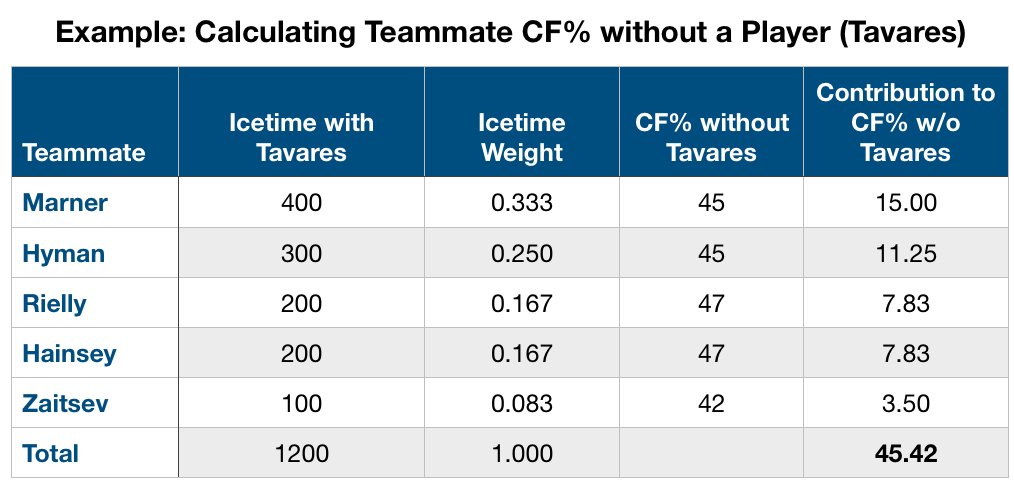
There are two basic steps in calculating a relative to teammates estimate. The table above is a simplified example of how the teammate portion is calculated.
First, see what each teammate’s ice time is and turn it into ice time weights that sum to 1.0 Marner is .333 because he played 400 minutes with Tavares out of 1200 total minutes.
Now multiply each teammate’s CF% without Tavares by that weight and total them up. In this example, the weighted teammate CF% without Tavares is 45.42%. If John Tavares’ CF% was 51%, then his ‘Relative to Teammates CF%’ would be
51%-45.42% = +5.58.
This approach has been shown to be a better way of isolating a player’s contributions in driving shot share than the more general on-ice CF%, or the more common relative to team versions.
3.3.5 Relative to Teammates Shots For
The relative to teammates change for CF (shot attempts for) is calculated the same way as shot share above.
3.3.6 Relative to Teammates Shots Against*
This statistic looks at the change in shots against for a team when a player is on the ice compared to the shots against when his teammates play without him in those games.
A player who is able to aid his teammates in preventing fewer 5v5 shots against on defense will score lower on this statistic. This is referred to as shot suppression and is one of the few defensive statistics in SKATR. The underlying shot xG estimates are from the MoneyPuck model.
*The percentile shown in SKATR is set up so that it gets closer to 100 as players suppress more shots against, relative to their teammates.
3.4 Context Stats
3.4.1 On-Ice xGF%
The expected goal share for a team when a player is on the ice and the sister statistic to on-ice CF% below. See Expected Goals in the Underlying Statistics section above for a general description of xG stats.
This statistic is based on the 10 players on the ice at 5v5, including the player. That is why it is placed in the Context section — it’s a multi-player statistic and is driven by the quality of teammates and opponents on the ice, not just the player. The relative to teammate version provides a better estimate of the player’s contribution to on-ice xGF%.
3.4.2 On-Ice CF%
Also referred to as “Corsi”, “shot share”, “possession”, or “shot differential”. CF% is simply the percentage of shot attempts taken by a player’s team at 5v5 when he/she is on the ice. This includes goals, missed shots, shots on goal and blocked shots. The intent is to help measure which team or player is driving play up ice more than the other direction and which player is on ice for what is *probably* more time in the offensive zone.
CF% = CF/(CF+CA) x 100.
Players will normally range between 40% and 60%, with most spread in between 45–55%. A value of 50% means that a player’s team is getting an equal share of shot attempts when the player is on the ice at 5v5.
CF% usually increases when trailing or playing at home so a score and venue adjusted version of CF% is used. This adjustment applies to all on-ice stats in SKATR.
If you keep in mind that a player is only one of ten skaters on the ice at 5v5, then you won’t over-interpret CF% at the player level. Context is important, especially the quality of teammates. In other words, playing with Patrice Bergeron has its benefits and it’s better to look at the relative to teammate version when assessing the player’s role in on-ice play-driving.
3.4.3 % Ice time
The TOI percentage of a team’s available 5v5 ice time played by a skater. If a team plays 48 minutes 5-on-5 and one defenseman plays 24 minutes, his TOI% is 50%. This helps define a player’s importance according to the coach. It is strongly correlated with Quality of Teammates.
3.4.4 Quality of Teammates
This is a weighted average of on-ice teammate quality based on their TOI%. It is probably the most important context indicator because teammates spend so much time together. If you are playing with the best defenseman in the league, chances are you get a boost.
3.4.5 % TOI vs Elite
In the last version of SKATR I used a standard Quality of Competition metric from Corsica. It was based on opponent TOI%. That metric spanned across many good and bad teams, coaching line choices, and players ranging from replacement to elite. This averaging washed away much of the information on competition.
It seemed a good opportunity to apply some form of segmentation of opposing players. I saw an opportunity to hopefully enhance our understanding of how often a player faces elite players. The source I found for that data was PuckIQ.com.
This article outlines the approach they took: to segment forwards into three “Woodmoney” tiers: “Elite”, “Middle”, and “Gritensity”.
Elite forwards were defined based on these rules:
1. Points/60 > 2.21 (all game states)
2. Time on ice per game > 75th percentile
3. Relative Corsi > 40th percentile
4. Relative Dangerous Fenwick* > 40th percentile
*Dangerous Fenwick is a version of unblocked shots that weighs shots by location and shot type. It is correlated with expected goals.
SKATR uses the percentage of ice time vs elite competition as a context indicator. It helps describe how a coach ranks a defenseman againt competition and gives an indication of how their on-ice and other results may be impacted. Cody Ceci’s results at the 91st percentile in “% TOI vs Elite” forwards is probably not going to be as high as it would be if he spent more time facing “Gritensity” forwards.
Here is an example showing Leafs defensemen using PuckIQ data. The defenseman with the highest DFF% ( a measure of dangerous shot share) is also the defenseman facing elite forwards the least (Travis Dermott).

3.4.6 Offensive Zone Start Ratio
This is the ratio of face-off starts in the offensive zone compared to the defensive zone.
OZ Start ratio = (DZFO/(DZFO+OZFO) x 100
If a defenseman is on for four face-offs in the OZ and one in the DZ, his ratio would be 80%. Don’t confuse OZ starts as necessarily a sign of defensive weakness in a player. Coaches will naturally put their best offensive players out more often for an OZ face-off.
Like other context variables, the OZ Start ratio is a barometer. It helps show how a coach prefers to use a player, but DZ and OZ face-offs represent a small proportion of a game’s total shift starts. They exclude neutral zone face-offs and the much more numerous on-the-fly shift changes. That limits how much we should conclude from this statistic.
Additional reading: How much do zone starts matter… (Matt Cane).
Conclusion
I hope you find this guide helpful in better understanding SKATR and hockey analytics as you explore NHL players. I believe the best analysts are those who look at players from all sides, are smart and humble enough to realize that numbers are only part of the story, and absorb what every source of information is telling them.
I want to thank again the public providers of hockey data who made SKATR possible. Your support of their sites and patreon accounts (and mine for that matter) will help keep public hockey data and visualizations thriving.
As SKATR changes and improves over time, so will this Guide. Any errors or omissions are my own. I also plan on writing a hockey analytics primer at some point in the future.
Finally, you can find examples of my use of SKATR and other data visualizations in my articles at MLHS. Here is one example.


